In this article, I’ll explain how to change the reference category of a factor variable in a linear regression in R.
The content of the page looks like this:
If you want to learn more about these content blocks, keep reading.
First, we need to create some example data that we can use in our linear regression:
set.seed(2580) # Create random example data N 1000 x sample(1:5, N, replace = TRUE) y round(x + rnorm(N), 2) x as.factor(x) data data.frame(x, y) head(data) # x y # 1 1 -1.93 # 2 3 3.15 # 3 2 0.14 # 4 1 1.33 # 5 1 0.11 # 6 3 3.60
As you can see based on the previous output of the RStudio console, our data consists of the two columns x and y, whereby each variable contains 1000 values. The variable x is a factor variable with five levels (i.e. 1, 2, 3, 4, and 5) and the variable y is our numeric outcome variable.
Now, we can apply a linear regression to our data:
summary(lm(y ~ x, data)) # Linear regression (default)
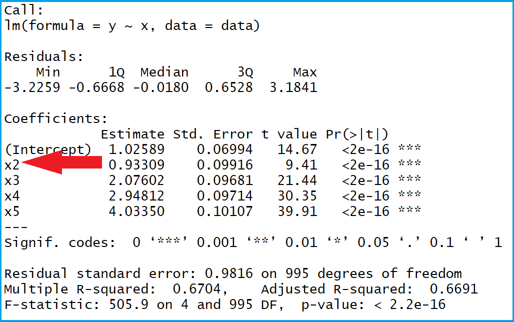
Table 1: Regular Output of Linear Regression in R.
Table 1 shows the summary output of our regression. As indicated by the red arrow, the reference category 1 was used for our factor variable x (i.e. the factor level 1 is missing in the regression output).
In the following example, I’ll show how to specify this reference category manually. So keep on reading!
If we want to change the reference category of a factor vector, we can apply the relevel function. Within the relevel function, we have to specify the ref argument to be equal to our desired reference category:
data$x relevel(data$x, ref = 2) # Apply relevel function
Now, let’s apply exactly the same linear regression R code as before:
summary(lm(y ~ x, data)) # Linear regression (relevel)
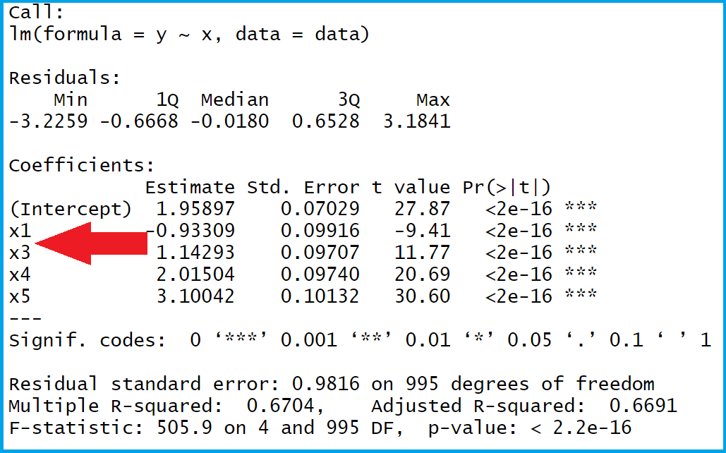
Table 2: Linear Regression Output with Modified Reference Category of Factor Variable.
Table 2 illustrates our summary statistics. As you can see, this time the reference category 2 was used (i.e. the factor level 2 is missing in the regression output). Looks good!
Have a look at the following video that I have published on my YouTube channel. In the video, I explain the content of this post:
In addition, you may want to read the other tutorials of this website:
Summary: In this article you learned how to force R to use a particular factor level as reference group in the R programming language. In case you have any additional comments and/or questions, let me know in the comments section.
set.seed(2580) N 1000 x sample(1:5, N, replace = TRUE) y round(x + rnorm(N, 1, 5), 2) # Increase noise x as.factor(x) data data.frame(x, y) summary(lm(y ~ x, data)) # Call: # lm(formula = y ~ x, data = data) # # Residuals: # Min 1Q Median 3Q Max # -14.9037 -3.2516 -0.1533 3.1922 16.1272 # # Coefficients: # Estimate Std. Error t value Pr(>|t|) # (Intercept) 2.1112 0.3544 5.957 3.55e-09 *** # x2 0.9625 0.5065 1.900 0.057693 . # x3 1.8316 0.4962 3.691 0.000235 *** # x4 2.5576 0.4893 5.227 2.10e-07 *** # x5 4.5836 0.4950 9.260 < 2e-16 ***# --- # Signif. codes: 0 ‘***’ 0.001 ‘**’ 0.01 ‘*’ 0.05 ‘.’ 0.1 ‘ ’ 1 # # Residual standard error: 4.936 on 995 degrees of freedom # Multiple R-squared: 0.0904, Adjusted R-squared: 0.08674 # F-statistic: 24.72 on 4 and 995 DF, p-value: < 2.2e-16data$x relevel(data$x, ref = 2) summary(lm(y ~ x, data)) # Call: # lm(formula = y ~ x, data = data) # # Residuals: # Min 1Q Median 3Q Max # -14.9037 -3.2516 -0.1533 3.1922 16.1272 # # Coefficients: # Estimate Std. Error t value Pr(>|t|) # (Intercept) 3.0737 0.3619 8.493 < 2e-16 ***# x1 -0.9625 0.5065 -1.900 0.05769 . # x3 0.8691 0.5016 1.733 0.08346 . # x4 1.5951 0.4948 3.224 0.00131 ** # x5 3.6210 0.5004 7.236 9.22e-13 *** # --- # Signif. codes: 0 ‘***’ 0.001 ‘**’ 0.01 ‘*’ 0.05 ‘.’ 0.1 ‘ ’ 1 # # Residual standard error: 4.936 on 995 degrees of freedom # Multiple R-squared: 0.0904, Adjusted R-squared: 0.08674 # F-statistic: 24.72 on 4 and 995 DF, p-value: < 2.2e-16Regards,

I’m Joachim Schork. On this website, I provide statistics tutorials as well as code in Python and R programming.